SPART Tutorial

This SPART tutorial will cover the basic operation of the library. Before starting make sure you have correctly installed and configured SPART (Installing SPART).

In this tutorial we will model the following spacecraft with a 5 degree-of-freedom manipulator with the following dimensions: L0=50, L1=125, L2=144, L3=47, L4=142, L5=80, L6=70 mm.

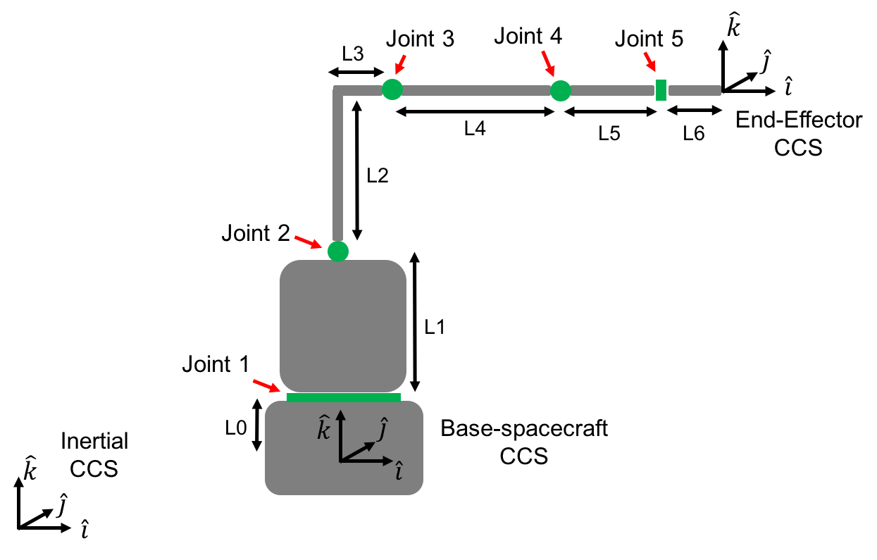
Spacecraft-manipulator system.

The code of this tutorial can be found in Examples/Tutorial/Tutorial.m.

Kinematics

Before SPART can start computing any kinematic or dynamic magnitude it needs a representation of the geometry and dynamic properties of the spacecraft-manipulator system. These fixed parameters are introduced into a data structure.

The data structure has 3 fields:

• data.n – Number of links.

• data.man(i) – Describes the ith link/joint.

  • data.man(i).type – Type of joint. 0 for a revolute joint, 1 for a prismatic joint.
  • data.man(i).DH – Denavit-Hartenberg parameters. Definitions are included below.
  • data.man(i).b – Vector from the Center-of-Mass of the link to the next joint in the local frame.
  • data.man(i).mass – Mass of the link.
  • data.man(i).I – Inertia matrix of the link.

• data.base – Describes the base-spacecraft.

  • data.base.T_L0_J1 – Homogeneous transformation matrix from the base to the first joint.
  • data.base.mass – Mass of the base-spacecraft.
  • data.base.I – Inertia matrix of the base-spacecraft

• data.EE – Provides additional information about the end-effector

  • data.EE.theta – Final rotation about the z axis. Last joint DH parameters are not enough to completely specify the orientation of the x and y end-effector axes.
  • data.EE.d – Final translation about the z axis. Last joint DH parameters are not enough to completely specify the location of the end-effector frame origin along the z-axis.

The kinematic relationship between a pair of connected joints is expressed by the Denavit-Hartenberg parameters.

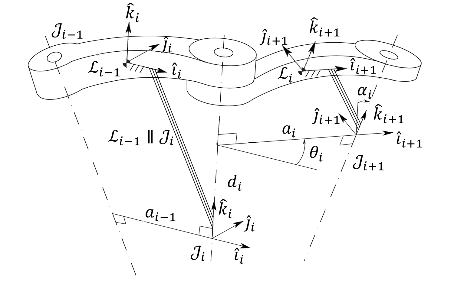
Denavit-Hartenberg parameters.

Denavit-Hartenberg parameters and their geometric definition.

Additional geometric definitions are included in the following figure.

Schematic disposition of links and joints.

The DH convention does not specify the orientation and origin of the first joint CCS (it’s origin must lie within the rotation or sliding axis). We then have freedom to set these. The orientation and the origin of the first joint are specified through the homogeneous transformation matrix data.base.T_L0_J1. An homogeneous transformation matrix encapsulates the orientation and position for a CCS with respect to another one, and in this particular case it can be written as follows.

\[\begin{split}^{\mathcal{L}_{0}}T_{\mathcal{J}_{1}}=\left[\begin{array}{cc} ^{\mathcal{L}_{0}}R_{\mathcal{J}_{1}} & ^{\mathcal{L}_{0}}s_{\mathcal{J}_{1}}\\ 0_{1,3} & 1 \end{array}\right]\end{split}\]

For this example we will assume that the base CCS and the first joint frame \(\mathcal{J}_{1}\) share the same orientation \(^{\mathcal{L}_{0}}R_{\mathcal{J}_{1}}=I_{3\times 3}\) and that \(\mathcal{J}_{1}\) is only displaced L0 in the \(k\) direction \(^{\mathcal{L}_{0}}s_{\mathcal{J}_{1}}=\left[0,0,L_{0}\right]^{T}\).

%Firts joint location with respect to base
data.base.T_L0_J1=[eye(3),[0;0;L0];zeros(1,3),1];

We will also assume that the links are homogeneous bodies and so their center-of-mass will be located at their geometric center, which allows to easily determine the data.man(i).b vector. The data.man(i).b vector goes from the center-of-mass of the ith link to the origin of the ith+1 joint in the local ith link reference frame. Using the DH parameters and assuming homogeneous bodies the DH and b vector are given below.

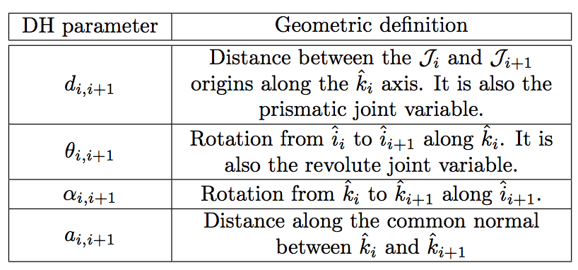
Joint/Link	DH.d	DH.alpha	DH.a	DH.theta	b
Joint 1	L1	pi/2	0	0	[0;L1/2;0]
Joint 2	0	0	sqrt(L2^2+L3^2)	atan2(L2,L3)	*see below
Joint 3	0	0	L4	–atan2(L2,L3)	[L4/2;0;0]
Joint 4	0	pi/2	0	pi/2	[0;0;–L5/2]
Joint 5	L5+L6	–pi/2	0	-pi/2	[L6/2;0;0]

data.man(2).b = [cos(-data.man(2).DH.theta),-sin(-data.man(2).DH.theta),0;sin(-data.man(2).DH.theta),cos(-data.man(2).DH.theta),0;0,0,1]*[L3^2/2;L2^2/2 + L3*L2;0]/(L2 + L3);

The resulting links and joints Cartesian Coordinate Systems are shown in the following image.

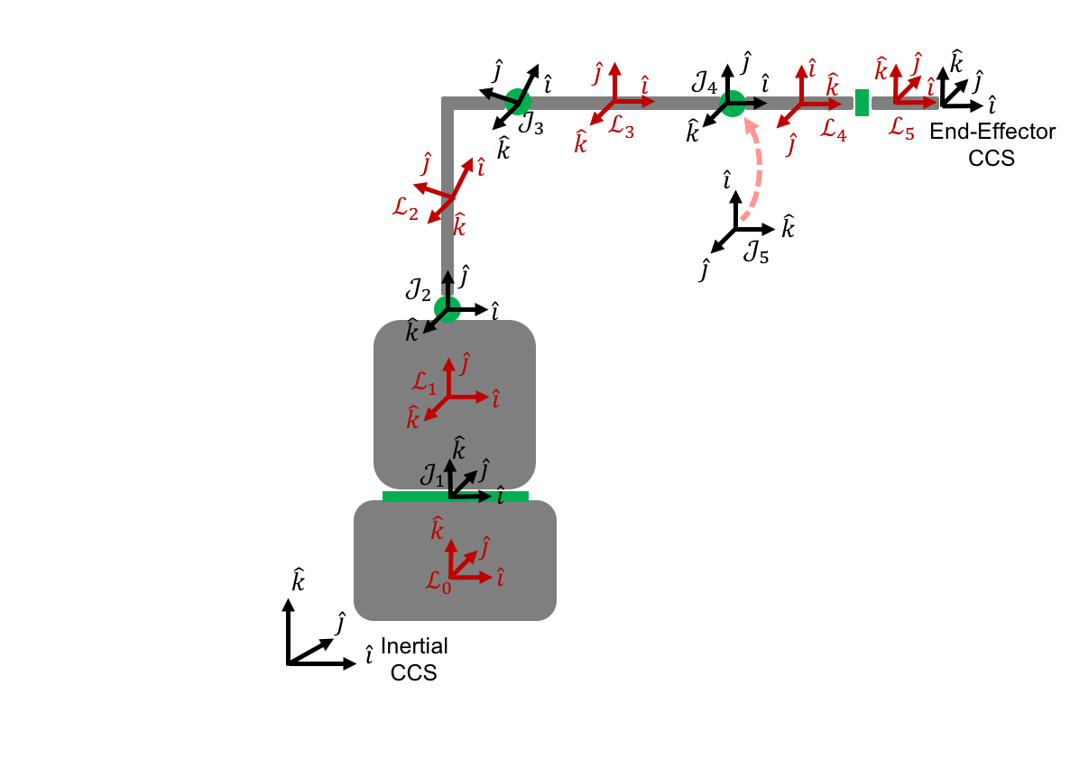
CCS of the spacecraft-manipulator system.

Finally, the DH parameters do not allow to freely set the end-effector CCS. For that we need two additional \(d\) and \(\theta\) DH parameters, that are applied to the last transformation. In this case the required values are as follows.

%End-Effector
data.EE.theta=-pi/2;
data.EE.d=0;

We can then create our data structure:

%--- Manipulator Definition ----%
%Number of joints/links
data.n=5;

%First joint
data.man(1).type=0;
data.man(1).DH.d = L1;
data.man(1).DH.alpha = pi/2;
data.man(1).DH.a = 0;
data.man(1).DH.theta=0;
data.man(1).b = [0;L1/2;0];

%Second joint
data.man(2).type=0;
data.man(2).DH.d = 0;
data.man(2).DH.alpha = 0;
data.man(2).DH.a = sqrt(L2^2+L3^2);
data.man(2).DH.theta=atan2(L2,L3);
data.man(2).b = [cos(-data.man(2).DH.theta),-sin(-data.man(2).DH.theta),0;sin(-data.man(2).DH.theta),cos(-data.man(2).DH.theta),0;0,0,1]*[L3^2/2;L2^2/2 + L3*L2;0]/(L2 + L3);

%Third joint
data.man(3).type=0;
data.man(3).DH.d = 0;
data.man(3).DH.alpha = 0;
data.man(3).DH.a =L4;
data.man(3).DH.theta=-atan2(L2,L3);
data.man(3).b = [L4/2;0;0];

%Fourth joint
data.man(4).type=0;
data.man(4).DH.d = 0;
data.man(4).DH.alpha = pi/2;
data.man(4).DH.a = 0;
data.man(4).DH.theta=pi/2;
data.man(4).b = [0;0;-L5/2];

%Fifth joint
data.man(5).type=0;
data.man(5).DH.d = L5+L6;
data.man(5).DH.alpha =-pi/2;
data.man(5).DH.a = 0;
data.man(5).DH.theta=-pi/2;
data.man(5).b = [L6/2;0;0];

%Firts joint location with respect to base
data.base.T_L0_J1=[eye(3),[0;0;L0];zeros(1,3),1];

%End-Effector
data.EE.theta=-pi/2;
data.EE.d=0;

Once the manipulator system has been defined we can then specify the configuration of the spacecraft manipulator system as follows.

%Base position
R0=eye(3);  %Rotation from base-spacecraft to the inertial frame
r0=[0;0;0]; %Position of the base-spacecraft in the inertial frame

%Joint variables [rad]
qm=[0;0;0;0;0];

Then we can start calling some functions. For example the kinematic function:

%Kinematics
[RJ,RL,r,l,e,g,TEE]=Kinematics_Serial(R0,r0,qm,data);

The output of the function is as follows:

• RJ – Joint 3x3 rotation matrices.
• RL – Links 3x3 rotation matrices.
• r – Links positions.
• l – Joints positions.
• e – Joints rotations axis.
• g – Vector from the origin of the ith joint to the ith link [inertial]
• TEE – End-Effector Homogeneous transformation matrix.

Now you can check that the r and l vectors provide the correct answers when qm=[0;0;0;0;0].

If you change the joint variables and re-run the kinematic function you will get the new positions with that particular configuration. The same can be done with the orientation R0 and position r0 of the base-spacecraft.

%Joint variables [rad]
qm=[45;10;-45;20;-90]*pi/180;

%Kinematics
[RJ,RL,r,l,e,g,TEE]=Kinematics_Serial(R0,r0,qm,data);

You can also define the joint variables as symbolic and obtain symbolic expressions.

%Joint variables [rad]
qm=sym('qm',[5,1],'real');

%Base-spacecraft position
r0=sym('r0',[3,1],'real');

%Base-spacecraft orientation
Euler_Ang=sym('Euler_Ang',[3,1],'real');
R0 = Angles321_DCM(Euler_Ang)';

%Kinematics
[RJ,RL,r,l,e,g,TEE]=Kinematics_Serial(R0,r0,qm,data);

Differential Kinematics

To compute the differential kinematics (including the Jacobians) can be computed if the base-spacecraft and joint velocities are specified.

%Velocities (joint space)
q0dot=zeros(6,1); %Base-spacecraft velocity
qmdot=[4;-1;5;2;1]*pi/180; %Joint velocities

%Differential Kinematics
[Bij,Bi0,P0,pm]=DiffKinematics_Serial(R0,r0,r,e,g,data);
%Velocities (operational space)
[t0,tm]=Velocities_Serial(Bij,Bi0,P0,pm,q0dot,qmdot,data);
%Jacobian of the Link 3
[J03, Jm3]=Jacob(r(1:3,3),r0,r,P0,pm,3,data.n);
%End-effector Jacobian
[J0EE, JmEE]=Jacob(TEE(1:3,4),r0,r,P0,pm,data.n,data.n);

The output of the differential kinematics as follows:

• t0 – Base–spacecraft twist vector [wx,wy,wz,vx,vy,vz].
• tm – Manipulator twist vector [wx,wy,wz,vx,vy,vz].
• Bij – Twist–propagation matrix (for manipulator i>0 and j>0).
• Bi0 – Twist–propagation matrix (for i>0 and j=0).
• P0 – Base–spacecraft twist–propagation vector.
• pm – Manipulator twist–propagation vector.

The twist vector encapsulates the angular and linear velocities in a vector.

\[\begin{split}t_{i}=\left[\begin{array}{c}\omega_{i}\\\dot{r}_{i}\end{array}\right]\end{split}\]

The twist vector can be propagated as follows from a link to the next using the 3x3 \(B_{ij}\) twist–propagation matrix and the 6x1 \(p_{i}\) twist–propagation vector as follows.

\[t_{i}=B_{ij}t_{j}+p_{i}\dot{q}_{i}\]

For the base-spacecraft the twist–propagation only uses the a modified 6x6 \(P_{0}\) twist-propagation vector.

\[t_{0}=P_{0}\dot{q}_{0}\]

Equations of Motion and inertia matrices

The generic equations of motion can be written as follows.

\[H\left(q\right)\ddot{q}+C\left(q,\dot{q}\right)\dot{q}=\mathcal{\tau}\]

With \(H\) being the generalized inertia matrix, \(C\) the generalized convective inertia matrix, \(q\) the generalized joint variables and \(\tau\) the generalized joint forces.

The generalized joint variables are composed by the base-spacecraft variables \(q_{0}\) and the manipulator joint variables \(q_{m}\). The contributions of the base-spacecraft and the manipulator can be made explicit when writing the equations of motion.

\[\begin{split}\left[\begin{array}{cc} H_{0} & H_{0m}\\ H_{0m}^{T} & H_{m} \end{array}\right] \left[\begin{array}{c} \ddot{q}_{0}\\ \ddot{q}_{m} \end{array}\right]+ \left[\begin{array}{cc} C_{0} & C_{0m}\\ C_{m0} & C_{m} \end{array}\right] \left[\begin{array}{c} \dot{q}_{0}\\ \dot{q}_{m} \end{array}\right]= \left[\begin{array}{c} \tau_{0}\\ \tau_{m} \end{array}\right]\end{split}\]

To obtain the inertia matrices we need to specify the mass and inertia of the base–spacecraft and of the joints.

Let’s assume, for the sake of simplicity, that all the links masses are 2 kg and have diagonal inertia matrices with \(I_{xx}=2/10\) kg/m2 \(I_{yy}=1/10\) \(I_{zz}=3/10\). And the base-spacecarft has a mass of 20 kg and inertia of \(I_{xx}=2\) kg/m2 \(I_{yy}=1\) \(I_{zz}=3\).

These variables can be added to the data structure as follows.

%First joint
data.man(1).mass=2;
data.man(1).I=diag([2,1,3])/10;

%Second joint
data.man(2).mass=2;
data.man(2).I=diag([2,1,3])/10;

%Third joint
data.man(3).mass=2;
data.man(3).I=diag([2,1,3])/10;

%Fourth joint
data.man(4).mass=2;
data.man(4).I=diag([2,1,3])/10;

%Fifth joint
data.man(5).mass=2;
data.man(5).I=diag([2,1,3])/10;

%Base-spacecraft mass and inertia
data.base.mass=20;
data.base.I=diag([2,1,3]);

You can now compute the inertia matrices as follows.

%Inertias in inertial frames
[I0,Im]=I_I(R0,RL,data);
%Mass Composite Body matrix
[M0_tilde,Mm_tilde]=MCB_Serial(I0,Im,Bij,Bi0,data);
%Generalized Inertia matrix
[H0,H0m,Hm]=GIM_Serial(M0_tilde,Mm_tilde,Bij,Bi0,P0,pm,data);
%Generalized Convective Inertia matrix
[C0,C0m,Cm0,Cm]=C_Serial(t0,tm,I0,Im,M0_tilde,Mm_tilde,Bij,Bi0,P0,pm,data);

Although the equations of motion can be used to solve the forward dynamic problem (determining the motion of the system given a set of applied forces \(\tau\rightarrow\ddot{q}\)) and the inverse dynamic problem (determining the forces required to produce a prescribe motion \(\ddot{q}\rightarrow\tau\)) there are more efficient ways of doing so.

Forward Dynamics

To solve the forward dynamics you will need to specify the forces acting on the spacecraft-manipulator system. There are two ways of specifying them and you can specify your forces in both of them if that is easier.

The joint forces \(\tau\) are the forces acting on the joints \(\tau_{m}\) (thus is an nx1 vector) and also at the base-spacecraft \(tau_{0}\) (thus a 6x1 vector). For \(\tau_{0}\), as in the twist vector, the torques come first and then the linear forces.

Also you can specify the wrenches \(w\) (torques and forces) for each body (applied at their center-of-mass). Again these can be decomposed into base-spacecraft 6x1 wrenches \(w_{0}\) and manipulator {6xn} wrenches \(w_{n}\).

Here is an example of how to do it.

%External forces
wF0=zeros(6,1);
wFm=zeros(6,data.n);

%Joint torques
tauq0=zeros(6,1);
tauqm=zeros(data.n,1);

Then a forward dynamic solver is available.

%Forward Dynamics
[q0ddot_FD,qmddot_FD] = FD_Serial(tauq0,tauqm,wF0,wFm,t0,tm,P0,pm,I0,Im,Bij,Bi0,q0dot,qmdot,data);

I you have forces that act on the links, for example gravity (with z being the vertical direction), they can be added through the wrenches as follows.

    %Gravity
    g=9.8; %[m s-2]

    %External forces (includes gravity and assumes z is the vertical direction)
    wF0=[0;0;0;0;0;-data.base.mass*g];
    wFm=[zeros(5,data.n);
-data.man(1).mass*g,-data.man(2).mass*g,-data.man(3).mass*g,-data.man(4).mass*g,-data.man(5).mass*g];

Inverse Dynamics

Similarly for the inverse dynamics the acceleration of the base-spacecraft and the joint need to be specified and then a function to compute the inverse dynamics is available.

%Accelerations
q0ddot=zeros(6,1);
qmddot=zeros(5,1);

%Accelerations
[t0dot,tmdot]=Accelerations_Serial(t0,tm,P0,pm,Bi0,Bij,q0dot,qmdot,q0ddot,qmddot,data);

%Inverse Dynamics - Flying base
[tau0,taum]=ID_Serial(wF0,wFm,t0,tm,t0dot,tmdot,P0,pm,I0,Im,Bij,Bi0,data);

If the base-spacecraft is left uncontrolled (floating case) and thus its acceleration is unknown a different routine is available.

%Accelerations
qmddot=zeros(5,1);

%Inverse Dynamics - Floating Base
[taum_floating,q0ddot_floating]=Floating_ID_Serial(wF0,wFm,Mm_tilde,H0,t0,tm,P0,pm,I0,Im,Bij,Bi0,q0dot,qmdot,qmddot,data);